The Lab-Wise File Drawer

The file drawer problem refers to a researcher failing to publish studies that do not get significant results in support of the main hypothesis. There is little doubt that file-drawering has been endemic in psychology. A number of tools have been proposed to analyze excessive rates of significant publication and suspicious patterns of significance (summarized and referenced in this online calculator). All the same, people disagree about how seriously the file-drawer distorts conclusions in psychology (e.g. Fabrigar & Wegener in JESP, 2016, with comment by Francis and reply). To my mind the greater threat of file-drawering noncompliant studies is ethical. It simply looks bad, has little justification in an age of supplemental materials that shatter the page count barrier, and violates the spirit of the APA Ethics Code.

But I’ll bet that all of us who have been doing research for any time have a far larger file drawer composed of whole lines of research that simply did not deliver significant or consistent results. The ethics here are less clear. Is it OK to bury our dead? Where would we publish whole failed lines of research?

Of course, some research topics are interesting no matter how they come out. As I’ve argued elsewhere, focusing on questions like these would remove a lot of uncertainty from careers and undercut the careerist motivation for academic fraud. But would even the most extreme advocate of open science reform back a hard requirement for a completely transparent lab?

The lab-wise file drawer rate — if you will, the circular file drawer — could explain part or all of publication bias. Statistical power could lag behind the near-unanimous significance of reported results due to whole lines of research being file-drawered. The surviving lines of research, even if they openly report all studies run, would then look better than chance would have it. I ran some admittedly simplistic simulations (Google Drive spreadsheet) to check out how serious the circular file drawer can get.

File, circular, quantity 1

 

Our simulated lab has eight lines of research going on, testing independent hypotheses with multiple studies. Each study has 50% power to find a significant result given the match between its methods and the actual, population effect size out there. You may think this is low, but keep in mind that even if you build in 80 or 90% power to find, say, a medium sized effect, the actual effect may be small or practically nil, reducing your power post-hoc.

The lab also follows rules for conserving resources while conforming to the standard of evidence that many journals follow. For each idea, they run up to three studies. If two studies fail to get a significant result, they don’t publish the research. They also stop the research short if either they fail to replicate a promising first study, or they try two studies, both of which fail. In this 50% power lab where each study’s success is a coin flip, this means that out of eight lines of research, they will only end up trying to publish three. Sounds familiar?

Remember, all these examples  assume that the lab reports even non-significant studies from lines of research that “succeed” by this standard. There is no topic-wise file drawer — only a lab-wise one.

In our example lab that runs at a consistent 50% power, at the spreadsheet’s top left, the results of this practice look pretty eye-opening. Even though not all reported results are significant, the 77.8% that are significant still exceed the 50% power of the studies. This leads to an R-index of 22, which has been described as a typical result when reporting bias is applied to a nonexistent effect (Schimmack, 2016).

Following the spreadsheet down, we see minimal effects of adopting slightly different rules that are more or less conservative in abandoning a research line after failure. They only require one study more or less about every 4 topics, and the R-indices from these analyses are still problematic.

Following the spreadsheet to the right, we see stronger benefits of carrying out more strongly powered research — which includes studying effects that are more strongly represented in the population to begin with. At 80% power, most research lines yield three significant studies, and the R-index becomes a healthy 71.

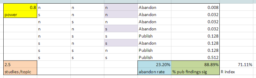
The next block to the right assumes only 5% power – a figure that breaks the assumptions of the R index. This represents a lab that is going after an effect that doesn’t exist, so tests will only be significant at the 5% type I error rate. Each of the research rules is very effective in limiting exposure to completely false conclusions, with only one in hundreds of false hypotheses making it to publication.

Before drawing too many conclusions about the 50% power example, however, it is important to question one of its assumptions. If all studies run in a lab have a uniform 50% power, and use similar methods, then all the hypotheses are true, with the same population effect size. Thus, variability in the significance of studies cannot reflect (nonexistent) variability in the truth value of hypotheses.

To reflect reality more closely, we need a model like the one I present at the very far right. A lab uses similar methods across the board to study a variety of hypotheses: 1/3 hypotheses with strong population support (so their standard method yields 80% power), 1/3 with weaker population support (so, 50% power), and 1/3 hypotheses that are just not true at all (so, 5% power). This gives the lab’s publication choices a chance to represent meaningful differences in reality, not just random variance in sampling.

What happens here?

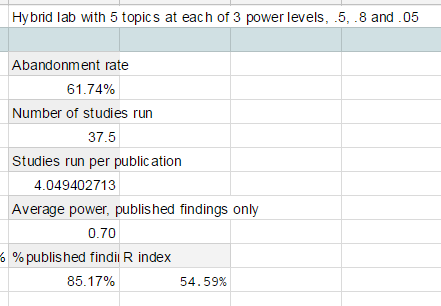
This lab, as expected, flushes out almost all of its tests of nonexistent effects, and finds relatively more success with research lines that have high power based on a strong effect, versus low power based on a weaker effect. As a result, inflation of published findings is still appreciable, but less problematic than if each study is done at a uniform 50% power.

To sum up:

1. A typical lab might expect to have its published results show inflation above their power levels even if it commits to reporting all studies relevant to each separate topic it publishes on.
2. This is because of sampling randomness in which topics are “survivors.” The more a lab can reduce this random factor — by running high-powered research, for example — the less lab-wise selection creates inflation in reported results.
3. A lab’s file drawer creates the most inflation when it tries to create uniform conditions of low power — for example, trying to economize by studying strong effects using weak methods and weak effects using strong methods, so that a uniform post-hoc power of 50% is reached (as in the first example). It may be better to let weakly supported hypotheses wither away (as in the hybrid lab example).

And three additional observations:

1. These problems vanish in a world where all results are publishable because research is done and evaluated in a way that reflects confidence in even null results (for example, the world of reviewed pre-registration). Psychology is a long way from that world, though.
2. The labwise file drawer adds another degree of uncertainty when trying to use post-hoc credibility analyses to assess the existence and extent of publication bias. Some of that publication bias may come from the published topic being simply more lucky than other topics in the lab.
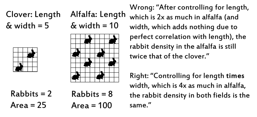
3. If people are going to disagree on the implications, a lot of it will hinge on whether it is ethical to not report failed lines of research. Those who think it’s OK will see a further reason not to condemn existing research, because part of the inflation used as evidence for publication bias could be due to this OK practice. Those who think it’s not OK will press for even more complete reporting requirements, bringing lab psychology more in line with practices in other lab sciences (see illustration).

   

   Being trusted is a privilege.

 

 

Quadratic Confounds, Linear Controls: A Doubt About That “Air Rage” Study

This past week it was hard to miss reading about the “air rage” study by Katherine DeCelles and Michael Norton, published in PNAS. They argued that economy-class passengers exposed to status inequalities when the flight had a first-class section were more likely to become belligerent or drunk — especially when the airplane boarded from the front and they had to walk right by those first-class 1%-ers in their sprawling leather seats. (article; sample news report).

Sounds compelling. But Andrew Gelman had doubts, based on some anomalies in the numbers and the general idea that it is easy to pick and choose analyses in an archival study. Indeed, for much research, one can level the critique that researchers are taking advantage of the “garden of forking paths”, but it’s harder to assess how much the analytic choices made could actually have influenced the conclusions.

This is where I found something interesting. In research that depends on multiple regression analysis, it’s important to compare zero-order and regression results. First, to see whether the basic effect is strong enough, so that the choices made for which variables to control for wouldn’t impact the results too much. Second, to see whether the conclusions being drawn from the regression line up with the zero-order interpretation of the effect that someone not familiar with regression would likely draw.

It’s already been remarked that the zero-order stats for the walk-by effect actually show a negative correlation with air rage; the positive relationship comes about only when you control for a host of factors. But the zero-order stats for the basic first-class air rage effect on economy are harder to get clear in the report. In the text, they are reported in raw, absolute numbers: over ten times as many air rage incidents occur on a yes/no basis in economy class when first class is present compared to when it is not. However, these raw numbers are naturally confounded by two factors that are highly correlated with the presence of a first class (see table S1 in the supplementary materials): length of flight and number of seats in economy. So you have to control for that in some way.

There was no data on actual number of passengers, but number of seats was used as a proxy for number of passengers, given that over 90% of flights are typically fully sold on that airline. In the article, number of seats and flight time are controlled for together, entered in the paper’s regression analysis on raw incident numbers per-flight. Not surprisingly, seats and time are correlated highly, nearly .80 (bigger planes fly longer routes), so including one after the other will not improve prediction much.

But most importantly, this approach doesn’t reflect that the effect of time and passenger numbers on behavioral base rates is multiplicative. That is, the raw amount of any kind of incident on a plane is a function of the number of people times the length of the flight, before any other factors like first class presence come into play. So what you need to do to model the rate of occurrence is  introduce an interaction term multiplying those two numbers – not just entering the two as predictors.

Or to put it another way – the analysis they reported might give a much lower effect of first class presence if they had taken as their outcome variable the proportion of air rage incidents per seat, per flight hour, because the outcome is still confounded with the size/length of the flight if you just control for the two of them in parallel.

Still confused? OK, one more time, with bunnies and square fields.

Although the data are proprietary and confidential, I would really appreciate seeing an analysis either controlling for the interaction of time and seats, or dividing the incidents by the product of time and number of seats before they go in as DVs, to arrive at the reasonable outcome of incidents per person per hour.

One other thing. Beyond their mere effects on base rates, long hours and many passengers may each affect raw numbers of air rage in a more exponential way – each with a quadratic function – by also leading to higher rates of incidents, even per person per hour, through higher numbers of potential interactions, and flight fatigue. So ideally, if you’re keeping raw numbers as the DV, the quadratic as well as linear functions of passenger numbers and flight time need to be modeled.

So the bottom line here for me is not that the garden of forking paths is in play, but that the wrong path appears to have been taken. I look forward to any feedback on this – especially from the authors involved.